C++ code for reading MNIST data-set

MNIST data-set is one of the most popular data-sets in the literature for testing deep learning algorithms performance. code for importing this data-set in MATLAB available here, however I could not find code for manipulating MNIST in C/C++. Reading it in C/C++ could be handy when you want to implement your deep learning algorithms in CUDA to boost the performance. I would like to mention that most portion of the code posted in the net by mrgloom.

#include <iostream>
#include <vector>

using namespace std;
int ReverseInt (int i)
{
    unsigned char ch1, ch2, ch3, ch4;
    ch1=i&255;
    ch2=(i>>8)&255;
    ch3=(i>>16)&255;
    ch4=(i>>24)&255;
    return((int)ch1<<24)+((int)ch2<<16)+((int)ch3<<8)+ch4;
}
void ReadMNIST(int NumberOfImages, int DataOfAnImage,vector<vector<double>> &arr)
{
	arr.resize(NumberOfImages,vector<double>(DataOfAnImage));
    ifstream file ("C:\\t10k-images.idx3-ubyte",ios::binary);
    if (file.is_open())
    {
        int magic_number=0;
        int number_of_images=0;
        int n_rows=0;
        int n_cols=0;
        file.read((char*)&magic_number,sizeof(magic_number));
        magic_number= ReverseInt(magic_number);
        file.read((char*)&number_of_images,sizeof(number_of_images));
        number_of_images= ReverseInt(number_of_images);
        file.read((char*)&n_rows,sizeof(n_rows));
        n_rows= ReverseInt(n_rows);
        file.read((char*)&n_cols,sizeof(n_cols));
        n_cols= ReverseInt(n_cols);
        for(int i=0;i<number_of_images;++i)
        {
            for(int r=0;r<n_rows;++r)
            {
                for(int c=0;c<n_cols;++c)
                {
                    unsigned char temp=0;
                    file.read((char*)&temp,sizeof(temp));
					arr[i][(n_rows*r)+c]= (double)temp;
                }
            }
        }
    }
}

int main()
{
  vector<vector<double>> ar;
  ReadMNIST(10000,784,ar);

  return 0;
}

Learning features for deep learning

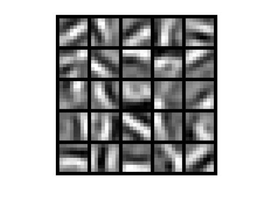
While ago I got introduced to the concept of deep learning while watching UCLA graduate summer school 2012 that can be found here. Unfortunately, I missed NN course offered by Geoff Hinton in Coursera which covers Deep Belief Nets, but I found two superb tutorials on deep learning one is UFLDL Stanford and Deeplearning.org website. In this post I add code of UFLDL first step of learning features by taking advantage of Autoencoders and escape any explanation since the tutorial itself has very well written and in depth description of concepts. The gist is to learn how to recreate input image by adding KL divergence as a penalty to NN cost function. Here is the code and result I got using data set provided in the tutorial:

Step 1: generating training set

for idx=1:numpatches
	rndimage = randperm(10);
	rndpixel = randi(504);
	rndy = randi(504);
	tmp = IMAGES(rndpixel:rndpixel+7,(rndy):(rndy)+7,rndimage(1));
	patches(:,idx) = tmp(:);
end

Step 2: Sparse autoencoder objective

KL = 0;
[n m] = size(data);
z2 = W1*data+repmat(b1,1,m);
a2 = sigmoid(z2);
z3 = W2*a2+repmat(b2,1,m);
a3 = sigmoid(z3);
ro = (1/m).*sum(a2,2);
KL = sum(sparsityParam.*log(sparsityParam./ro)+(1-sparsityParam).*log((1-sparsityParam)./(1-ro)));
cost = (0.5/m)*sum(sum((a3-data).^2))+lambda*(1/2)*(sum(sum(W1.^2))+sum(sum(W2.^2)))+beta*KL;
d3 = -(data-a3).*sigmoidGradient(z3);
betaterm = beta*(-sparsityParam./ro+(1-sparsityParam)./(1-ro));
d2 = (W2'*d3+repmat(betaterm,1,m)).*sigmoidGradient(z2);
W1grad = W1grad+d2*data';
W1grad = (1/m)*W1grad+lambda*W1;
W2grad = W2grad+d3*a2';
W2grad = (1/m).*W2grad+lambda*W2;
b1grad = b1grad+sum(d2,2);
b1grad = (1/m)*b1grad;
b2grad = b2grad+sum(d3,2);
b2grad = (1/m)*b2grad;

Step 3: Gradient checking

e = 1e-4;
for p = 1:numel(theta)
   perturb(p) = e;
   numgrad(p) = (J(theta + perturb) - J(theta - perturb)) / (2*e);
   perturb(p) = 0;
end

Here are the learned features

weights

Google search engine version 0.0

I was busy during these month with amazing Prof’s NG ML course in coursera and from now on direction of this blog bends through machine learning. After getting interested in ML I Googled to find more courses about this subject and came across very help full Porf. Freitas class in UBC  and decided to work on his class assignments while watching class videos which are available in youtube.

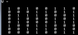
As you can check in assignments and first couple of lectures the assignment is to implement a search engine based on Google algorithm. The main idea of this algorithm is that linking between webpages can be represented in a binary matrix form consisting ob bunch of ones representing there is a link between two webpages and 0 otherwise as shown in the following figure:

Webpages matrix

Webpages matrix

After that to avoid reducibility, we add small value say 0.001, to all elements of matrix. resulting to the following matrix:

Adding epsilon to avoid reducibility

Adding epsilon to avoid reducibility

After that we convert this matrix to stochastic matrix, means each row of matrix summed to one. this can be done by dividing each element of the row by the sum of the elements which leads to the following matrix:

Stochastic matrix

Stochastic matrix

Here is the gist of the algorithm, we create an stochastic arbitrary vector of size of the matrix (here the size is 8) and multiply it with the matrix several time until it converges and stop changing, this vector can simply be one divided by number of pages ([1/8,1/8,1/8,1/8,1/8,1/8,1/8,1/8]). the resulting vector is our (well its Google’s) page rank. In case of this example the vector converges to:

Page rank

Page rank

And we are done! we just implemented Google search engine (but version 0.0), following is the complete python code of the assignment using webpages provided as class logistics:

</pre>
#!/usr/bin/env python

import numpy as np
import numpy.random as npran
import networkx as nx
import matplotlib.pyplot as plt
import pickle as pk
import numpy.linalg as lin
from numpy import sum

def getPageRank(fname):
 return R[0,f2i[fname]]

links = {}
fnames = ['angelinajolie.html', 'bradpitt.html','jenniferaniston.html', 'jonvoight.html','martinscorcese.html', 'robertdeniro.html']

for file in fnames:
 links[file] = []
 try:
 with open(file): f = open(file)
 except IOError:
 print ('Oh dear.')

 for line in f.readlines():
 while True:
 p = line.partition('<a href="http://')[2]
 if p=='':
 break
 url, _, line = p.partition('\">')
 links[file].append(url)
 f.close()

DG = nx.DiGraph()
DG.add_nodes_from(fnames)
edges = []
for key, values in links.items():
 eweight={}
 for v in values:
 if v in eweight:
 eweight[v] +=1
 else:
 eweight[v]=1
 for succ, weight in eweight.items():
 edges.append([key, succ, {'weight':weight}])

DG.add_edges_from(edges)

plt.figure(figsize=(9,9))
pos=nx.spring_layout(DG)
nx.draw(DG,pos,node_size=0,alpha=0.4,edge_color='r',font_size=14)
plt.savefig("link_graph.png")
plt.show()

pk.dump(DG, open('DG.pkl','wb'))

NX = len(fnames)

T = np.matrix(np.zeros((NX,NX)))

f2i = dict((fn, i) for i, fn in enumerate(fnames))

for predecessor, successors in DG.adj.items():
 for s, edata in successors.items():
 T[f2i[predecessor], f2i[s]] = edata['weight']

epsilon = 0.01

E = np.ones(T.shape)/NX
L = T + epsilon * E
G = np.matrix(np.zeros(L.shape))
for i in range(6):
 G[i,:] = L[i,:] / sum(L[i,:])

PI = npran.random(NX)
PI /= sum(PI)
R = PI
for _ in range(100):
 R = np.dot(R, G)
evolution = [np.dot(PI, G**i) for i in range(1, 20)]
plt.figure()
for i in range(NX):
 stp = [step[0,i] for step in evolution]
 plt.plot(stp,label=fnames[i], lw=2)

plt.title('rank vs iterations')
plt.xlabel('iterations')
plt.ylabel('rank')
plt.legend()
plt.show()

revind = {}
for fname in fnames:
 for line in open(fname).readlines():
 for token in line.split():
 if token in revind:
 if fname in revind[token]:
 revind[token][fname] += 1
 else:
 revind[token][fname] = 1
 else:
 revind[token] = {fname: 1}

print(revind['the'])
result = revind['the'].keys()
print(sorted(result, key=getPageRank, reverse=True))
<pre>

For some reason spaces disappear when I copy and paste the code, copying and pasting exact code will most probably gives you indentation error. you need to fix that in order to run the code.

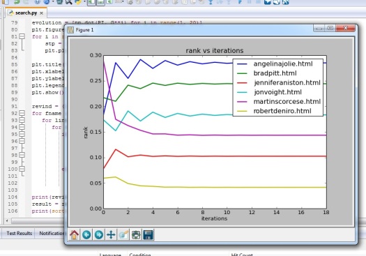
Here is ranking results:

final

Image blending using pyramid

In the previous post I discussed about image pyramid and how to build them. one of the use of image pyramid is making you able to blend two images so it appear to be natural. I got the idea while watching this  a lecture on image pyramids by Prof.Shah.

The method is straight forward the code takes the two images and a mask, and splits them into their channels. It then blends each channel separately. The code will build laplacian pyramid for the images and then build a gaussian pyramid for the mask. At the end, it blend the two pyramids and collapse them down to the output image.

here are the functions in the code and explanation:

  1. Reduce: This function takes an image and out put it’s quarter size by dividing the height and width by two.
  2. Expand: This function takes an image and out put it’s four times size by doubling the height and width by two.
  3. Gaussian PyramidThis function takes an image as an input and builds its pyramid and return the result as an array. The first member of the array is the original image and other members of the array are reduced form of the previous member.
  4. Laplacian PyramidThis function takes a gaussian pyramid array from the previous function, and return an array containing laplacian pyramid.
  5. BlendThis function takes three arrays of laplacian pyramid two images and a gaussian pyramid of a mask image, then it performs blending of the two laplacian pyramids using mask pyramid weights.
  6. CollapseThis function accepts a laplacian pyramid, then it takes the top layer, expand it, and then add it to the next layer this process continues until a single image remain and this will be returned as a result.

Here is the complete code:

import sys
import os
import numpy as np
import cv2
import scipy
from scipy.stats import norm
from scipy.signal import convolve2d
import math
'''split rgb image to its channels'''
def split_rgb(image):
  red = None
  green = None
  blue = None
  (blue, green, red) = cv2.split(image)
  return red, green, blue

'''generate a 5x5 kernel'''
def generating_kernel(a):
  w_1d = np.array([0.25 - a/2.0, 0.25, a, 0.25, 0.25 - a/2.0])
  return np.outer(w_1d, w_1d)

'''reduce image by 1/2'''
def ireduce(image):
  out = None
  kernel = generating_kernel(0.4)
  outimage = scipy.signal.convolve2d(image,kernel,'same')
  out = outimage[::2,::2]
  return out

'''expand image by factor of 2'''
def iexpand(image):
  out = None
  kernel = generating_kernel(0.4)
  outimage = np.zeros((image.shape[0]*2, image.shape[1]*2), dtype=np.float64)
  outimage[::2,::2]=image[:,:]
  out = 4*scipy.signal.convolve2d(outimage,kernel,'same')
  return out

'''create a gaussain pyramid of a given image'''
def gauss_pyramid(image, levels):
  output = []
  output.append(image)
  tmp = image
  for i in range(0,levels):
    tmp = ireduce(tmp)
    output.append(tmp)
  return output

'''build a laplacian pyramid'''
def lapl_pyramid(gauss_pyr):
  output = []
  k = len(gauss_pyr)
  for i in range(0,k-1):
    gu = gauss_pyr[i]
    egu = iexpand(gauss_pyr[i+1])
    if egu.shape[0] > gu.shape[0]:
       egu = np.delete(egu,(-1),axis=0)
    if egu.shape[1] > gu.shape[1]:
      egu = np.delete(egu,(-1),axis=1)
    output.append(gu - egu)
  output.append(gauss_pyr.pop())
  return output
'''Blend the two laplacian pyramids by weighting them according to the mask.'''
def blend(lapl_pyr_white, lapl_pyr_black, gauss_pyr_mask):
  blended_pyr = []
  k= len(gauss_pyr_mask)
  for i in range(0,k):
   p1= gauss_pyr_mask[i]*lapl_pyr_white[i]
   p2=(1 - gauss_pyr_mask[i])*lapl_pyr_black[i]
   blended_pyr.append(p1 + p2)
  return blended_pyr
'''Reconstruct the image based on its laplacian pyramid.'''
def collapse(lapl_pyr):
  output = None
  output = np.zeros((lapl_pyr[0].shape[0],lapl_pyr[0].shape[1]), dtype=np.float64)
  for i in range(len(lapl_pyr)-1,0,-1):
    lap = iexpand(lapl_pyr[i])
    lapb = lapl_pyr[i-1]
    if lap.shape[0] > lapb.shape[0]:
      lap = np.delete(lap,(-1),axis=0)
    if lap.shape[1] > lapb.shape[1]:
      lap = np.delete(lap,(-1),axis=1)
    tmp = lap + lapb
    lapl_pyr.pop()
    lapl_pyr.pop()
    lapl_pyr.append(tmp)
    output = tmp
  return output

def main():

 image1 = cv2.imread('c:/apple.jpg')
 image2 = cv2.imread('c:/orange.jpg')
 mask = cv2.imread('c:/mask512.jpg')
 r1= None
 g1= None
 b1= None
 r2= None
 g2= None
 b2= None
 rm= None
 gm = None
 bm = None

 (r1,g1,b1) = split_rgb(image1)
 (r2,g2,b2) = split_rgb(image2)
 (rm,gm,bm) = split_rgb(mask)

 r1 = r1.astype(float)
 g1 = g1.astype(float)
 b1 = b1.astype(float)

 r2 = r2.astype(float)
 g2 = g2.astype(float)
 b2 = b2.astype(float)

 rm = rm.astype(float)/255
 gm = gm.astype(float)/255
 bm = bm.astype(float)/255

 # Automatically figure out the size
 min_size = min(r1.shape)
 depth = int(math.floor(math.log(min_size, 2))) - 4 # at least 16x16 at the highest level.

 gauss_pyr_maskr = gauss_pyramid(rm, depth)
 gauss_pyr_maskg = gauss_pyramid(gm, depth)
 gauss_pyr_maskb = gauss_pyramid(bm, depth)

 gauss_pyr_image1r = gauss_pyramid(r1, depth)
 gauss_pyr_image1g = gauss_pyramid(g1, depth)
 gauss_pyr_image1b = gauss_pyramid(b1, depth)

 gauss_pyr_image2r = gauss_pyramid(r2, depth)
 gauss_pyr_image2g = gauss_pyramid(g2, depth)
 gauss_pyr_image2b = gauss_pyramid(b2, depth)

 lapl_pyr_image1r  = lapl_pyramid(gauss_pyr_image1r)
 lapl_pyr_image1g  = lapl_pyramid(gauss_pyr_image1g)
 lapl_pyr_image1b  = lapl_pyramid(gauss_pyr_image1b)

 lapl_pyr_image2r = lapl_pyramid(gauss_pyr_image2r)
 lapl_pyr_image2g = lapl_pyramid(gauss_pyr_image2g)
 lapl_pyr_image2b = lapl_pyramid(gauss_pyr_image2b)

 outpyrr = blend(lapl_pyr_image2r, lapl_pyr_image1r, gauss_pyr_maskr)
 outpyrg = blend(lapl_pyr_image2g, lapl_pyr_image1g, gauss_pyr_maskg)
 outpyrb = blend(lapl_pyr_image2b, lapl_pyr_image1b, gauss_pyr_maskb)

 outimgr = collapse(blend(lapl_pyr_image2r, lapl_pyr_image1r, gauss_pyr_maskr))
 outimgg = collapse(blend(lapl_pyr_image2g, lapl_pyr_image1g, gauss_pyr_maskg))
 outimgb = collapse(blend(lapl_pyr_image2b, lapl_pyr_image1b, gauss_pyr_maskb))
 # blending sometimes results in slightly out of bound numbers.
 outimgr[outimgr < 0] = 0
 outimgr[outimgr > 255] = 255
 outimgr = outimgr.astype(np.uint8)

 outimgg[outimgg < 0] = 0
 outimgg[outimgg > 255] = 255
 outimgg = outimgg.astype(np.uint8)

 outimgb[outimgb < 0] = 0
 outimgb[outimgb > 255] = 255
 outimgb = outimgb.astype(np.uint8)

 result = np.zeros(image1.shape,dtype=image1.dtype)
 tmp = []
 tmp.append(outimgb)
 tmp.append(outimgg)
 tmp.append(outimgr)
 result = cv2.merge(tmp,result)
 cv2.imwrite('c:/blended.jpg', result)

if  __name__ =='__main__':
 main()

Here is the result

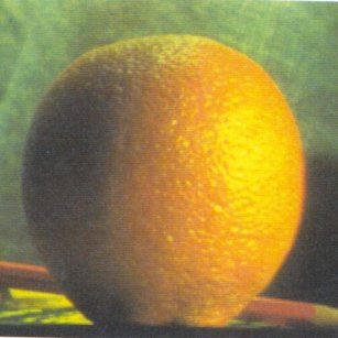
Two images to be blended:

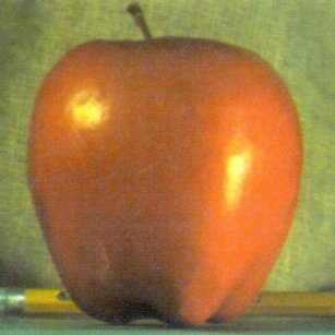
orange

apple


Mask:

mask512


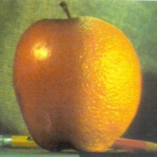
Result:

blended

Image pyramids – Theory

Image pyramids is one of the most used tools in image processing since it allow us to capture image features in different scales. There are two basic functionality used in building pyramids: reduce operation and expand. reduce will used to re size the image down by half and expand is to double the size of the image.

By adding the reduced image on top of each other a pyramid will be constructed as shown below:

Simply removing one pixel out of two wouldn’t be a good choice for reduce since we may loos important information or capture a noise. Therefore smoothing (Gaussian) before reducing is inevitable. By doing this we simply build a Gaussian pyramid. Another well-known pyramid is Lablacian pyramid, for building this pyramid, say level 1, we should subtract Gaussian level 1 from expanded Gaussian level 2, the result will be Laplacian level 1. It should be noted that the last Laplacian level is identical to the last level of Gaussian pyramid.

So the algorithm for building Gaussian pyramid is:

1-Smooth the image with Gaussian filter

2-Sub sample the image by half

3-If reached desired size stop, else send the result to step 1

Algorithm for Laplacian is:

1-Build a Gaussian pyramid

2-Until last element of Gaussian pyramid not reach do:

2-1 ith Laplacian pyramid = ith Gaussian pyramid – expanded of (i+1)th Gaussian pyramid

Convolution – OpenCV

Convolution probably is the most used method in field of image processing in order to apply a certain mask (kernel) to the image. Here  is a good explanation about convolution. Its simply multiplying mask’s values with image’s pixels intensity and sum them up as show below:

Adapted from apple.com

However it should be noticed that because of taking care of impulse response the kernel should be flipped horizontally and vertically.  Here is code for applying convolution on an image:


def convolve(image, kernel):
  '''fliping kernel'''
  rkernel=np.rot90(kernel,2)
  '''creating output image based on input image dimention
  notice that I did not take care of the image edges
  so out put will has less pixels than orginal, the number
  of omitted pixels depends on kernel size'''
  output = np.zeros((1+image.shape[0]-kernel.shape[0],1+image.shape[1]-kernel.shape[1]), dtype=image.dtype)
  for i in range(0,output.shape[0]):
   for j in range(0,output.shape[1]):
    signal_patch = image[i:i+kernel.shape[0],j:j+kernel.shape[1]]
    tmp = (rkernel * signal_patch).sum()
	'''not really the best method to normalize the image'''
    if tmp>255:
     tmp=255
    if tmp<0:
     tmp=0
    output[i,j]=tmp
  return output

Computational Photography course in coursera

This week Computational Photography course in coursera.org, which I enrolled last month, started. The instructor is Prof.Irfan Essa from Georgia tech. Assignments of the first week were kinda easy, RGB channel spiting which I blogged about it before, convert to gray scale and image reconstructing (use to 300×800 images to create 600×800 image). Optional assignments seems more challenging though.

By the way, good thing about this course is that I can get familiar with using OpenCV in python.

Here is the code for the image reconstructing:

def interlace(evens, odds):
outimg = None

'''outimg = (np.random.rand(evens.shape[0]+odds.shape[0],evens.shape[1],evens.shape[2])*0).astype(np.uint8)'''
outimg = np.zeros((evens.shape[0]+odds.shape[0], evens.shape[1],evens.shape[2]), dtype=np.uint8)
outimg[0::2,:,:]=evens
outimg[1::2,:,:]=odds
return outimg

note that evens and odds variables should be numpy arrays.

Evens image:

even

Odds image:

odd

Result:

together


Seam carving – MATLAB

While reading course materials for computer vision in different universities I found  out a very interesting algorithm for image size changing called “seam carving” can be found here. The power of this algorithm is that unlike other re-sizing methods here content of the image is trying to be take care of in other word its content-aware.

Here is a video clip showing its power and applicability


First energy of the image calculated, this could be simply image gradient. Then we calculate the sum of each column’s pixel energy value (its absolute value) -this can be done for each row as well – then at the bottom of the image we find the smallest value. Considering dynamic programming we back track from the minimum value to the top of the image, where in each step we have to chose the smallest three upper values. A very good explanation with a step by step illustration can be found in Wikipedia.

Here I implemented seam carving method to find vertical seam, same method can be used to find horizontal seams as well. As before, the code is not optimized and just used for testing purpose.

function [ output_args ] = SeamCarving(I)

%   Detailed explanation goes here
%calculating image gradient as an energy image
[rmax, cmax,tmp] = size(I);
img = double(I)/255;
img = rgb2gray(img);
[Ix,Iy]=gradient(img);
Gimg=Ix+Iy;
Gimg=abs(Gimg);
%calculating sum of pixels value in each column
test2=zeros(rmax,cmax);
for row = 1 :rmax
    for col = 1:cmax
        if row == 1
            test2(row,col)=Gimg(row,col);
        end
        if row>1
            if col ==1
                tmp=[test2(row-1,col),test2(row-1,col+1)];
                test2(row,col)= Gimg(row,col)+min(tmp);
            end
            if col>1 && col<cmax
                tmp1=[test2(row-1,col),test2(row-1,col+1),test2(row-1,col-1)];
                test2(row,col)= Gimg(row,col)+min(tmp1);
            end
            if col == cmax
                tmp2=[test2(row-1,col),test2(row-1,col-1)];
                test2(row,col)= Gimg(row,col)+min(tmp2);
            end
        end
    end
end
minval=min(test2(rmax,:));
locations=find(test2(rmax,:)==minval);
[x,y]=size(locations);
%back traking to find the seam
for loc=1:y
    j = locations(1,loc);
    for row=rmax:-1:1
        if row==rmax
            I(row,j,1)=255;
            I(row,j,2)=0;
            I(row,j,3)=0;
        end
        if row < rmax
            if j==1
                tmp=[test2(row+1,j),test2(row+1,j+1)];
                [C,index]=min(tmp);
                if index==1
                    I(row+1,j,1)=255;
                    I(row+1,j,2)=0;
                    I(row+1,j,3)=0;
                end
                if index==2
                    I(row+1,j+1,1)=255;
                    I(row+1,j+1,2)=0;
                    I(row+1,j+1,3)=0;
                    j=j+1;
                end
            end
            if j>1 && j<cmax
                tmp1=[test2(row+1,j),test2(row+1,j+1),test2(row+1,j-1)];
                [C,index]=min(tmp1);
                if index==1
                    I(row+1,j,1)=255;
                    I(row+1,j,2)=0;
                    I(row+1,j,3)=0;
                end
                if index==2
                    I(row+1,j+1,1)=255;
                    I(row+1,j+1,2)=0;
                    I(row+1,j+1,3)=0;
                    j=j+1;
                end
                if index==3
                    I(row+1,j-1,1)=255;
                    I(row+1,j-1,2)=0;
                    I(row+1,j-1,3)=0;
                    j=j-1;
                end
            end
            if j == cmax
                tmp2=[test2(row+1,j),test2(row+1,j-1)];
                [C,index]=min(tmp2);
                if index==1
                    I(row+1,j,1)=255;
                    I(row+1,j,2)=0;
                    I(row+1,j,3)=0;
                end
                if index==2
                    I(row+1,j-1,1)=255;
                    I(row+1,j-1,2)=0;
                    I(row+1,j-1,3)=0;
                    j=j-1;
                end
            end
        end
    end
end
imshow(I);
end

Here is the output:

OpenCV Basics – Splitting RGB channels

Lets back to basics..splitting RGB channels in OpenCV can be done using split function. Note that the function returns RGB in reverse order (BGR). Here is the code. Additionally same code can be used to get HSV and YCrCb as well, as you can see in commented section. cheers

#include <iostream>
#include <string>
#include <iomanip>
#include <sstream>

#include <opencv2/imgproc/imgproc.hpp>
#include <opencv2/core/core.hpp>
#include <opencv2/highgui/highgui.hpp>

using namespace std;
using namespace cv;

int main(int argc, char *argv[]){
	VideoCapture capture("c://video.avi");
	Mat frame;
	while(true){
		if(!capture.read(frame)){
			break;
		}
		Mat output (frame.size(),frame.type());
		vector<Mat> rgb;
		//vector<Mat> hsv;
		//vector<Mat> ycrcb;
		//cvtColor(frame,output,CV_RGB2YCrCb);
		namedWindow("Orginal");
		imshow("Orginal", frame);
		// split(frame, rgb);
		split(frame, rgb);

		namedWindow("b");
		namedWindow("g");
		namedWindow("r");

		imshow("b", rgb[0]);
		imshow("g", rgb[1]);
		imshow("r", rgb[2]);

		if(waitKey(25)>=0)
			break;
	}
	waitKey(0);
}

Harris interest point detection – Implementation (OpenCV)

After discussing Harris corner detection in last post  now lets see how we can implement it after implementation we compare our result with OpenCV built in Harris corner detection.

first lets see how built in Harris function in OpenCV works and what Its result. This function in OpenCV called cornerHarris and accepts following parameters:

void cornerHarris(InputArray src, OutputArray dst, int blockSize, int ksize, double k, int borderType=BORDER_DEFAULT );

Where details about parameters can be found here. Now lets see what would be the result of using this function using following code (sample retrieved from here).

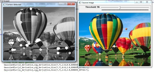
Here you can see the result of cornerHarris function in OpenCV using threshold 96. now lets write our own Harris corner detection (would appreciate it if anyone can point out any mistake I might have).

#include "opencv2/highgui/highgui.hpp"
#include "opencv2/imgproc/imgproc.hpp"
#include <iostream>
#include <stdio.h>
#include <stdlib.h>

using namespace cv;
using namespace std;

char* source_window = "Source image";
char* corners_window = "Corners detected";
Mat src,x2y2, xy,mtrace,src_gray, x_derivative, y_derivative,x2_derivative, y2_derivative,
	xy_derivative,x2g_derivative, y2g_derivative,xyg_derivative,dst,dst_norm, dst_norm_scaled;
int thresh = 128;

void onTrackbar( int, void* );

int main( int argc, char** argv )
{
	//Get Image
	src = imread( "f:/samples/balloon_small.bmp");
	//Create window to show source image
	namedWindow( source_window, CV_WINDOW_AUTOSIZE );
	//Create trackbar to change threshold
	createTrackbar( "Threshold", source_window, &thresh, 255, onTrackbar);

	//Show source image
	imshow( source_window, src );
	onTrackbar(thresh,0);

	waitKey(0);
	return(0);
}

void onTrackbar( int, void* ){
	cvtColor( src, src_gray, CV_BGR2GRAY );
	//Step one
	//to calculate x and y derivative of image we use Sobel function
	//Sobel( srcimage, dstimage, depthofimage -1 means same as input, xorder 1,yorder 0,kernelsize 3, BORDER_DEFAULT);
	Sobel(src_gray, x_derivative, CV_32FC1 , 1, 0, 3, BORDER_DEFAULT);
	Sobel(src_gray, y_derivative, CV_32FC1 , 0, 1, 3, BORDER_DEFAULT);
	//Step Two calculate other three images in M
	pow(x_derivative,2.0,x2_derivative);
	pow(y_derivative,2.0,y2_derivative);
	multiply(x_derivative,y_derivative,xy_derivative);
	//step three apply gaussain
	GaussianBlur(x2_derivative,x2g_derivative,Size(7,7),2.0,0.0,BORDER_DEFAULT);
	GaussianBlur(y2_derivative,y2g_derivative,Size(7,7),0.0,2.0,BORDER_DEFAULT);
	GaussianBlur(xy_derivative,xyg_derivative,Size(7,7),2.0,2.0,BORDER_DEFAULT);
	//forth step calculating R with k=0.04
	multiply(x2g_derivative,y2g_derivative,x2y2);
	multiply(xyg_derivative,xyg_derivative,xy);
	pow((x2g_derivative + y2g_derivative),2.0,mtrace);
	dst = (x2y2 - xy) - 0.04 * mtrace;
	//normalizing result from 0 to 255
	normalize( dst, dst_norm, 0, 255, NORM_MINMAX, CV_32FC1, Mat() );
	convertScaleAbs( dst_norm, dst_norm_scaled );
	// Drawing a circle around corners
	for( int j = 0; j < src_gray.rows ; j++ )
		{ for( int i = 0; i < src_gray.cols; i++ )
			{
				if( (int) dst_norm.at<float>(j,i) > thresh )
				{
					circle( src_gray, Point( i, j ), 5,  Scalar(255), 2, 8, 0 );
				}
			}
		}
  // Showing the result
  namedWindow( corners_window, CV_WINDOW_AUTOSIZE );
  imshow( corners_window, src_gray );
}

I tried to comment the code appropriately and define each step in Harris algorithm so it can be self-explaining but most probably not as optimal as it could be. Here is the result of using threshold 96 using our Harris corner detector.

hcorner

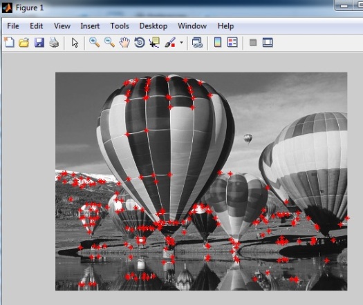
As you can see there are some difference in detection which I couldn’t figure it out why its like this, even built in  function of Harris detector in MATLAB produce slightly different results as you can see in the following figure, although I couldn’t figure it out how to specify threshold in MATLAB.

harrismatlab